Companding

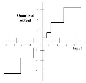
In previous experiment we considered an Analog to Digital Converter (ADC) where the quantizer was uniformly spaced against amplitude axis. This allows uniform resolution or step size for the entire range of the signal. The resulting error or quantization noise is also same for all the amplitude levels. While this appears to be a very logical way of quantizing signal if quantization error / noise is perceived uniformly across all amplitude levels, there are occasions when it is not actually so. For example, human auditory system follows what can be related to a logarithmic process in which high amplitude sounds do not require the same resolution as low amplitude sounds. The human ear is more sensitive to quantization noise in small amplitude signals than the large ones

Companding is combination of two terms compressing and expanding. In the context of quantization, this refers to compressing the higher amplitude signal first through a non-uniform quantization process and then expanding it to get back the signal. To obtain non-uniform quantization a two step process may be followed - first pass the signal through a compressor and then compress it by a uniform quantizer (discussed in second experiment).

In speech coding, in an attempt to follow the human auditory system A-law and mu-law companding are used. Both apply logarithmic quantization functions to adjust the bit resolution in proportion to the level of the input signal. Smaller signals are represented with greater precision or more data bits and larger signals with less data bits. The result is fewer bits per sample to maintain an audible signal-to-noise ratio (SNR). Note the term 'audible'. Audible SNR is the perceived SNR and not actual SNR.

The sampled discrete time signal x(nT) , n=0,1,2,.... of the original continuous time signal x(t) is shown in Fig. 2 below.

For computational ease, A-law and m-law companding match logarithmic curve with a piece-wise linear approximation. This first sets eight straight-line segments along the curve to produce a close approximation to the logarithm function. Each segment is known as a chord. Within each chord, the piece-wise linear approximation is divided into equally size quantization intervals called steps. The step size between adjacent codewords is doubled in each succeeding chord. Also encoded is the sign bit for the original integer. The result is an 8-bit logarithmic code composed of a 1-bit sign bit, a 3-bit chord, and a 4-bit step.

A-Law Compander

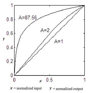
A-law is the CCITT recommended companding standard that is used across Europe and rest of the countries except Japan, Canada and North America. Limiting the linear sample values to 12 magnitude bits, the A-law compression is defined by Equation 1, where A is the compression parameter (A=87.7 in Europe), and x is the normalized signal to be compressed.

$$ \left(\begin{array}{cc} A \frac{|x|}{1+ln A} & |x|<\frac{1}{A}\ 1+\frac{ln(A|x|)}{(1+ln(A)} & \frac{1}{A}<=|x|<=1 \end{array}\right) ..............(1)$$

μ-Law compander

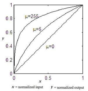
The United States and Japan use m-law companding. In that, the linear sample values are limited to 13 magnitude bits, the m-law compression is defined by Equation 2, where μ is the compression parameter (μ =255 in the U.S. and Japan) and x is the normalized signal to be compressed.

$$y=sgn(x) \frac{ln(1+\mu|x|)}{ln(1+\mu)}, -1<=x<=1....(2)|$$

The companding process for m-law is similar to that of A-law. The major differences are: (i) μ-law encoders typically operate on linear 13-bit magnitude data, as opposed to 12-bit magnitude data with A-law, (ii) before chord determination a bias value of 33 is added to the absolute value of the linear input data to simplify the chord and step calculations, (iii) the definition of the sign bit is reversed, and (iv) the inversion pattern is applied to all bits in the 8-bit code

In this experiment, we use this equation and allow you (the students) to choose number of bits and understand how A-law companding is used in quantization. The aim is to make you understand non-uniform quantization and not the format of the data presentation.